Excel pivot table tutorial - How To Discuss
Excel pivot table tutorial
How to create classic pivot table in Excel? Part 1 of 3. Creating a pivot table Load the worksheet from which you want to create a pivot table. You can use a pivot table to visually represent the data in a table. Make sure your data meets the pivot table requirements. The pivot table is not always the answer you want. Start the PivotTable Wizard. Select the data you want to use.
How do you open a pivot table in Excel?
Steps Start Microsoft Excel. Open the pivot table and data file. Make the necessary adjustments to the original data. Select the workbook sheet that contains the pivot table by clicking the appropriate tab. Click in the PivotTable to open the PivotTable Tools menu. Change the source data range for the pivot table.
How do I create a pivot table in Microsoft Excel?
To create a PivotTable, open Microsoft Excel, enter the data in the worksheet, select all the data, and select PivotTable on the Insert tab at the top of the screen. Create a pivot table in this free desktop video and capture a variety of data and fields with the help of a software developer's IT department. Video of the day.
How do I learn pivot tables in Excel?
At the beginning of this tutorial, you'll learn how to insert a pivot table into a sample Excel sheet. Select all dates in the worksheet. Click the Insert tab on the Excel ribbon and click the PivotTable button. The Create PivotTable dialog box appears. Click OK to insert an empty pivot table into the new worksheet.
How do you create a pivot table in Excel?
Click the Design button. Now drag the fields you want to appear in the Side, Row, Column, and Data sections of the pivot table. In this example, they will drag the Order ID field to the Product section and the Quantity field to the Data section. Click OK to continue. Now click on the Finish button.
Where do I find the PivotTable button in Excel?
Go to Insert > Pivot Table. If you're using Excel for Mac 2011 and earlier, the PivotTable button is on the Data tab in the Analyze group. Excel displays the Create PivotTable dialog box with the selected table name or range.
 How can I change the layout of the pivot table?
Right-click a cell in the PivotTable to display the context menu and select PivotTable Options. See screenshot: 2. In the PivotTable Options dialog box, click the View tab and select the Classic PivotTable Layout check box (allows you to drag fields on the grid). See screenshot: 3. Click OK to close the dialog box, and the PivotTable layout will now change.
 How to create a 2 dimensional pivot table in Excel?
2D Pivot Tables 1 Activate the sales table. 2 Click the ENTER tab. 3 Click the PivotChart button and select Table 4. Select All Data. Excel should now remember the old range so all you need to do is click OK 5 Create a new sheet using the pivot table tools 6 Select the fields as shown in the image below.
 How to create classic pivot table in excel tutorial
Create a PivotTable 1 Select the cells from which you want to create a PivotTable. 2 Choose Insert > Pivot Table. 3 Under Select data to analyze, select Select table or range. 4 In the table / range, check the cell range.
How to set Classic pivot table layout in Excel?
In the Save As dialog box, select the folder where you want to save the workbook, and then select Excel Workbook 972003 from the Save as type list. See screenshot: 3. Click Save to close the dialog box. Then PivotTables that you insert in the workbook in the future will be automatically displayed as Classic PivotTables.
How to create a PivotTable to analyze data?
In the Select data to analyze section, select Select table or range. Check cell range in table/range. Under Choose where to place the PivotTable report, select New Sheet to place the PivotTable on a new or existing sheet, and then select where to place the PivotTable.
 What are pivot tables used for?
- View large amounts of data in a variety of easy-to-use ways.
- Subtotals and aggregated numerical data, summarize data by category and subcategory and create your own calculations and formulas.
- Expand and collapse data layers to focus results and explore detailed summary data for areas of interest.
How do you build a pivot table?
Creating a PivotTable Load the worksheet from which you want to create a PivotTable. Make sure your data meets the pivot table requirements. Start the PivotTable Wizard. Select the data you want to use. Choose a location for your pivot table.
 Which is the best source for a PivotTable?
Tables are an excellent source of PivotTable data because rows added to the PivotTable are automatically added to the PivotTable when the data is refreshed, and new columns are added to the PivotTable's Field List. Otherwise, you must modify the original data in the PivotTable or use a formula with a named dynamic range.
 How to create a pivot table in excel
1. Click a cell in the pivot table. 2. On the Analysis tab, in the Tools group, click PivotChart. The "Insert Chart" dialog box appears. 3. Click OK. Below is a summary table. This pivot table will surprise and impress your boss.
 How do you add a custom column to a pivot table?
From the drop-down menu, click Calculated Field. A new window will open where you can add a new custom column to the pivot table. In the Name box, enter a name for the column. Click in the Name field and enter the name you want to use for the new column.
 What are the best uses of pivot tables?
Pivot tables are most commonly used in situations where data needs to be merged, split, and collapsed for analysis. This is especially useful when you want to calculate and summarize data for comparison.
 How do you collapse a pivot table in Excel?
Click the expand/collapse button to the left of the pivot element header OR double-click the cell with the header. The Collapse and Expand (or double-click) buttons affect all instances of the pivot function.
 How to create classic pivot table in excel sheet
Select a table or range on the worksheet, then choose Insert > PivotTable. The Insert PivotTable area shows the data source and destination where the PivotTable will be inserted, as well as recommended PivotTables. To manually create a pivot table, select Create your own pivot table.
 How to change the format of a PivotTable in Excel?
On the Analysis or Parameters tab, in the PivotTable group, click Parameters. In the PivotTable Options dialog box, click the Layout and Formatting tab, and then under Format, do one or more of the following: To change the way errors are displayed, select the Show values for check box. In the box, enter the value to display in place of errors.
When would you use VLOOKUP in Excel?
Excel's VLOOKUP function can be used when you need to find values in a specific table and compare them to other data fields for comparison. VLOOKUP stands for vertical search, which is used to find specific data from a data table.
 What you should know about Excel VLOOKUP?
23 things to know about VLOOKUP How VLOOKUP works is a function you can use to find and retrieve data in a table. VLOOKUP just looks good. Perhaps the biggest limitation of VLOOKUP is that it can only see the data correctly. VLOOKUP finds the first match. If the lookup column contains duplicate values in exact match mode, VLOOKUP matches only the first value.
How do I use the V-lookup formula on Excel?
- Click on Formula tab > Find and reference > click on vlookup.
- Also click the function icon, then type manually and search for the formula.
- You will get a new function window as below pictures show.
- Then you need to fill in the details as the picture shows.
- Place the lookup value where you want to map one table to another table value.
 Why is my VLOOKUP not working properly?
The main reason why vlookup doesn't work is because the numbers in your cells are actually text. They look like numbers, you could even format them and format them as numbers. but trust me, it's still text.
 How do you sort pivot tables in Excel?
Follow these steps to sort in Excel Desktop. In the pivot table, click the small arrow next to the Row Labels and Column Labels cells. Click the field for the row or column you want to sort. Click the arrow for the row or column labels, then select the desired sorting option. To sort the data in ascending or descending order, click Sort A to Z or Sort Z to A.
 How do I add pivot tables in Excel?
Follow the instructions below to insert a pivot table. 1. Click on any cell in the dataset. 2. On the Insert tab, in the Tables group, click PivotTable. The following dialog box appears. Excel automatically selects the dates for you. The default location for a new pivot table is New Worksheet.
What is a pivot table template?
Follow the steps below. Specify the data range. If your data is in a worksheet range, just select a cell in that range. Select cell A2 on your datasheet. Create an empty pivot table. Click OK to leave the settings unchanged. Excel creates an empty PivotTable and displays the PivotTable Fields task pane. Customize pivot table.
Where to find pivot table in Excel 2016?
Excel 2016 for dummies. On the Analyze tab, click the PivotTable Tools contextual tab to see the buttons on your ribbon. In the Show group, click the Field List button. Excel displays the PivotTable Field List task pane, which lists the fields that are currently in the PivotTable and the ranges to which they are mapped.
 How to enable show details in PivotTable in Excel?
To find the source data table, you can use the Enable detail display in a pivot table feature. 1. Right-click a cell in the pivot table and select PivotTable Options from the context menu. See screenshot: 2. In the dialog box that appears, click the Data tab, and then select the Include display details option. See screenshot: 3.
 How to consolidate multiple PivotTables in Excel 2016?
Open the file in Excel 2016. Select ALT + D, then P and the PivotTable / PivotChart Wizard opens. Select multiple consolidation areas. Select a PivotTable or PivotChart report.
 How do you insert a pivot table in Excel?
To do this, select all of your data (including column headings), click Insert on the ribbon, and then click the PivotTable button. 3. Select where you want to place the pivot table. After clicking the PivotTable button, you will see a popup asking where you want to place the PivotTable.
How to show field list in pivot table?
To display a list of fields in an Excel PivotTable: 1 First, select a cell in the PivotTable. 2 On the ribbon, click the Analysis / Parameters tab. The tab is called Options in Excel 2010 and earlier. 3 Click the Field List button on the right side of the ribbon. It is also a toggle button that shows or hides the list of fields.
 How do you highlight the first row of a pivot table in Excel?
Just highlight the first row of your data, click the Data tab on the ribbon, click Filter, and then click the arrow that appears in the column header to see all the items in that column. Obviously, this technique is best for more manageable data sets.
 How do you open a pivot table in excel for dummies
If you want to delete the pivot table and leave other items on the sheet intact, you can delete the cells. 1. Select a cell in the pivot table. 2. Click Change | in the menu bar. Delete | Everything. 3. On the PivotTable toolbar, click PivotTable | Select | The whole table. This will remove the pivot table and all formatting from the worksheet.
How do I calculate a pivot table?
Steps Start Microsoft Excel. Open a worksheet containing the PivotTable and the raw data you are working with. Select the worksheet tab with the original data. Define the calculation you want to add. Add a column for the calculated differences. Enter a name for the column, such as B.
 How to build your pivot tables?
- Clean up your data. Before creating anything in Excel, it's a good idea to take a quick look at your data to make sure everything looks right.
- Insert a pivot table. Believe it or not, we've reached the point where you can add a pivot table to your workbook.
- Choose where to place the pivot table.
How to unique count in a pivot table?
Counting Unique Values in a PivotTable Follow these steps to count unique values in a PivotTable. Note: This unique account is only valid if you have Excel 2016 or higher (download sample data).
How do you open a pivot table in excel worksheet
Click a cell on the sheet. Click Insert > Pivot Table. In the Create PivotTable dialog box, under Select data to analyze, click Use an external data source.
How do you open a pivot table in excel sheet
Start the PivotTable Wizard. At the top of the Excel window, click the Insert tab. Click the PivotTable button on the left side of the Insert ribbon.
How do I refresh all PivotTables in Excel?
To update a single pivot table, you can right-click anywhere in the pivot table area and select Update. If you have multiple pivot tables, first select a cell in a pivot table, then go to the pivot table analysis on the ribbon > click the arrow below the refresh button and select Refresh All.
How do you open a pivot table in excel definition
Go to the INSERT tab and click on the PivotTable - the Create PivotTable dialog box will open and if you have not selected a region, the entire table/range will be automatically selected as the data you want to analyze - at this point, you click just click OK and the new pivot table will be added to the new worksheet, just like on the Excel desktop.
How to create a pivot table in microsoft excel
Let's get started and combine the data. To open the PivotTable and Chart Wizard, press Alt + D + P, select multiple consolidation areas, and click Next. In the next step of the wizard, select the "Create a page for me" field and click the "Next" button. Now select the areas you want to combine.
 How do you combine multiple tables in Excel?
Here are the steps to combine multiple sheets with Excel spreadsheets using Power Query: Click the Data tab. In the Get Data and Transform group, click Get Data. Go to the "From other sources" option. Click the Empty query option. The Power Query Editor opens.
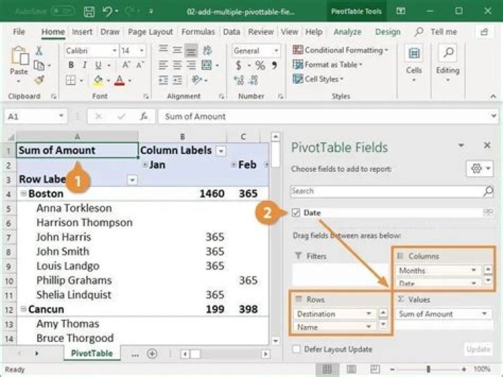
What is pivot in Excel?
- Strings: data used as a specification.
- Values: number of dates.
- Filter: Filter to hide certain data.
- Columns: values in different conditions.
How do you create a pivot?
How to make a pivot table. Enter data in a series of rows and columns. Sort the data according to specific criteria. Highlight your cells to create a pivot table. Drag the field to the Row Labels area. Drag the field to the values area.
 How do I create pivot table from multiple sheets?
How to make a pivot table from multiple sheets. An easy way is to use the PivotTable and PivotChart wizards. To enable it, click Options on the File tab, click Customize Ribbon, select All commands in the Select commands from: box, and scroll down until you find the Pivot Cross Chart Wizard and click yours. Click on "Add >>".
What is the importance of pivot tables?
A pivot table is a data synthesis tool used in the context of data processing. Pivot tables are stored in the database to summarize, sort, rearrange, group, count, total, or average. It allows users to convert columns to rows and rows to columns.
How do I sort pivot table by values in Excel?
To sort a pivot table by value, select the value in the column and sort it as you would in any Excel spreadsheet. You can do the same with the commands. Let's analyze in descending order. As always, you can mouse over the rating icon to see the currently used rating options.
How do I create pivot table from multiple sheets in Excel?
Start the PivotTable and Chart Wizard by pressing Alt + D, P and selecting Multiple Consolidation Areas. Select > I will create page fields and click Next. Now select the area for the data where you want to create the pivot table and also select the column headings.
 How do I analyze a pivot table in Excel?
First of all, you need to create a pivot table in Excel. You will then learn to analyze trends using pivot tables. To do this, follow these steps: Click a cell in the table. Then go to the "Insert" tab. Then click the pivot table button. Finally, click OK.
 Apakah Microsoft Excel membutuhkan pivot table?
Microsoft Excel sebenarnya sudah menyediakan fitur classification (pengurutan data), filtered (penyaringan data) subtotal Serta (pengelompokan data dan perhitungan) table pada sebuah, namun jika anda merasa fitur atau fasilitas tadi masutih kurang maka sepatin.
Mengapa Anda menggunakan PivotTable pada Excel?
Menggunakan pivot table keywords in excel. Sebelum anda mengetahui langkah apa saja dalam menggunakan fitur Pivot table pada pekerjaan anda dalam menggunakan MS. excel, anda harus tahu dahulu tentang manfaat pivot table ini, yaitu. Membuat pengelompokan data yang berdasarkan kategori sesuai yang diinginkan.
Apa yang digunakan untuk membuat pivot table?
Fitur's dropfield area cannot be used for pivot tables that use the striping function to use different methods. Fitur ini memungkinkan pengguna dapat menentukan urutan baris table and column table dengan melakukan drag. Digunakan zone filter for menampilcan, store data pivot table.
 Apakah Anda perlu menerapkan format Table pada tabel pivot Anda?
Seperti yang sud di jelaskan di atas, sangat disarankan format table Leadapkan Pada Sumber Data Pivot anda. Salah satu kelebihannya adalah and mempermudah melakukan update the data of jika sumber yan anda gunakan untuk table Pivot merupakan sebuah data yan dinamis atau berubah setiap saat.
 How do pivot tables in Excel work?
Every pivot table in Excel starts with a simple Excel spreadsheet that stores all your data. To create this table, place your values in a specific set of rows and columns. Use the top row or top column to sort the values by what they represent.
 Excel pivot table tutorial mac
1. Click a cell in the source data or table area. 2. Go to Insert > Pivot Table. If you're using Excel for Mac 2011 and earlier, the PivotTable button is on the Data tab in the Analyze group. 3. Excel displays the Create PivotTable dialog box with the selected range or table name.
How do you find pivot tables in Excel?
To get a PivotTable, click the Insert tab and find the PivotTable option in the Tables group. Microsoft Excel 2007/2010/2013/2016/2019 hides the PivotChart Wizard, which does not appear on the ribbon. This function is not so intuitive to obtain without the classic Excel menu.
How to create a two dimensional pivot table in Excel?
2D PivotTable By dragging a field to the row area and column area, you can create a 2D PivotTable. First add the pivot table. Then drag the fields below into different sections to export the total to each country and product.
What can pivot tables do for your business?
He estimates that by leveraging the power of pivot tables with the ubiquitous Sage software, the entire account creation process can be reversed, accounts can take up to 25% less time, better reporting management, and better reporting.